The problem with a single number
Consider a five-year plan that projects a 22% equity IRR. The number is the product of a dozen assumptions — revenue growth, margin expansion, an exit multiple, a discount rate — each entered as a single value the analyst believes is reasonable. The trouble is that "reasonable" is not the same as "certain." Revenue growth of 8% is a reasonable estimate, but so is 5%, and so is 12%. The model does not know that. It takes 8%, runs it through, and returns 22% with the same confident precision it would give a physical constant.
This is sometimes called the flaw of averages: a model built entirely on best-guess midpoints returns a best-guess midpoint, and that midpoint systematically misrepresents anything with a non-linear payoff. A deal that returns 22% at the base case might return 30% if a few things break right and go underwater if a few break wrong — and the asymmetry between those two tails is exactly the information an investment committee, a board, or a lender needs. A point estimate throws it away.
Analysts have always known this, which is why they build scenarios and sensitivity tables. Those are good tools and this guide is not an argument against them. But a base/bull/bear stack still only shows you three futures out of a near-infinite set, and a sensitivity table shows you one or two inputs moving at a time. Neither answers the question a risk-aware decision-maker actually asks: across everything that could plausibly happen, what is the distribution of outcomes, and how much of it is bad?
What Monte Carlo simulation actually is
Strip away the intimidating name and the method is simple. Instead of entering each uncertain assumption as one number, you enter it as a range with a shape — a probability distribution. Revenue growth is no longer "8%"; it is "normally distributed, centered on 8%, with most of the mass between 5% and 11%." Then the computer does something a human never could by hand: it draws one random value from each input's distribution, runs the entire model, records the outputs, and repeats — thousands of times.
Each run is called a trial. After ten thousand trials you no longer have one IRR; you have ten thousand of them, and their histogram is the answer. It tells you the median outcome, the shape of the upside, the depth of the downside, and — most valuably — the probability of any threshold you care about. What is the chance IRR falls below the 15% hurdle? Count the trials below 15% and divide by ten thousand. That is the whole idea. The name comes from the Monte Carlo casino, because the engine underneath is nothing more than repeated random sampling.
The one-sentence version: a point estimate answers "what is the most likely outcome?" — Monte Carlo answers "what is the full range of outcomes, and how likely is each?" The second question is the one with money riding on it.
The anatomy of a simulation: inputs, trials, outputs
Every Monte Carlo has three parts, and getting each one right is the whole craft.
1. Inputs — the assumptions you make uncertain
You do not turn every cell into a distribution. Most of a model's inputs barely move the answer, and randomizing them just adds noise. The inputs worth simulating are the two, three, or four load-bearing assumptions — the ones a sensitivity analysis has already flagged as high-impact. If you have not done that sensitivity pass first, do it before you simulate; it tells you where to spend your uncertainty budget. (Our guide to sensitivity analysis beyond two variables covers how to find those drivers.)
2. Trials — the repeated random draws
Each trial draws one value from each input distribution and recalculates the model end to end. The number of trials determines how smooth and stable your output is. Too few and the tails are noisy; too many wastes time for no added accuracy. For nearly all business models, somewhere between 1,000 and 10,000 trials is the right range — more on that below.
3. Outputs — the distribution and its percentiles
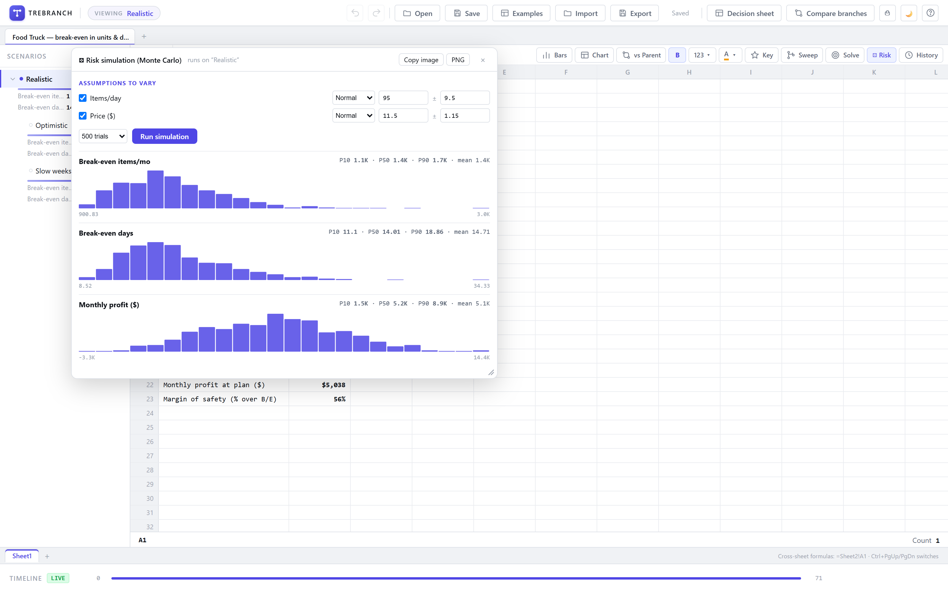
The output is a distribution, usually shown as a histogram, and it is summarized by percentiles. The three that matter most are P10, P50, and P90:
- P50 (the median): half the trials came out below this, half above. This is your central estimate — and notice it is often not equal to the base-case point estimate, especially when the model has any non-linearity.
- P10: only 10% of trials fell below this. It is your realistic downside — not the worst case imaginable, but the bad outcome you should genuinely plan for.
- P90: 90% of trials fell below this. Your realistic upside.
The gap between P10 and P90 is the single most useful thing the simulation produces, because it is the width of the range your point estimate was hiding. Two projects can share an identical P50 and be completely different investments if one has a tight P10–P90 band and the other has a wide one. That difference is invisible to a single-number model and obvious in a distribution.
A convention trap: in oil, gas, and mineral reserves, the percentile convention is often reversed — P90 is the conservative, high-confidence figure and P10 is the optimistic one. In most corporate finance and FP&A work the convention is as described above (P10 low, P90 high). Whenever you share percentiles across teams, state which direction you mean.
Choosing the right distribution
Analysts new to simulation agonize over distribution choice, but in practice three shapes cover the vast majority of business assumptions. The goal is not statistical perfection — it is an honest representation of what you actually know.
| Distribution | Use when | Typical inputs |
|---|---|---|
| Normal | Values cluster symmetrically around a central estimate, extremes are unlikely | Cost inflation, a mature product's growth rate, wage growth |
| Triangular | You can name a minimum, most-likely, and maximum but not the precise shape | A ramp period, a new market's adoption, a construction timeline |
| Uniform | Any value in a range is equally plausible; you have no basis to favor the middle | A regulatory outcome, a price you truly cannot handicap |
The triangular distribution is the workhorse of practical modeling precisely because it maps to how humans actually estimate: "it will probably take nine months, but it could be as fast as six or as slow as fifteen." That sentence is a triangular distribution. You do not need to know standard deviations to use it, which is why it dominates project finance and operational modeling.
A final principle: getting the range roughly right matters far more than getting the shape exactly right. An honest triangular estimate with a realistic spread will serve you better than a mathematically elegant distribution anchored too tightly on the base case. The most common failure is not choosing the wrong curve — it is choosing a spread that is too narrow because the modeler could not bring themselves to imagine the assumption being very wrong.
Where Monte Carlo earns its keep
Probabilistic modeling is not an academic curiosity; it is standard practice wherever the cost of being wrong is large and the future is genuinely uncertain.
- Insurance and reinsurance. Actuaries have priced catastrophe and long-tail liability risk with simulation for decades — the entire discipline of reserving assumes the future is a distribution, not a number.
- Energy and project finance. Majors run oil-price decks and demand forecasts through thousands of paths to test whether a multi-decade asset stays solvent across the range, not just at the planning-case price. The same logic underpins how lenders stress a project's debt-service coverage ratio.
- Aerospace and large programs. Cost-and-schedule risk simulation is how organizations running complex programs — NASA among them — set the confidence level of a budget, answering "what number do we need so there is only a 30% chance of overrun?" rather than quoting a single point estimate.
- Private equity and credit. Beyond the named downside case, simulation quantifies the probability that a deal misses its return hurdle or trips a covenant, which is a sharper question than "does the bear case still work?"
- Pharma and R&D. The value of a drug candidate or a research program is inherently a distribution across trial outcomes and adoption curves; a single risk-adjusted NPV hides the shape that actually drives the go/no-go.
The common thread is that each of these decisions is dominated by uncertainty, and each has a payoff that is asymmetric — the downside and upside are not mirror images. That is exactly the situation a point estimate handles worst and a distribution handles best.
The Excel problem
Native Excel does not do Monte Carlo well. You can force it — a RAND()-driven input, a one-column data table with a few thousand rows to hold the trial results, and some percentile formulas — but it is slow, it recalculates unpredictably, it clutters the model with simulation scaffolding, and it does not scale past a couple of outputs before it becomes unmanageable. Anyone who has built one knows it is a fragile piece of machinery.
The traditional answer is a dedicated add-in — @RISK from Palisade or Crystal Ball from Oracle. Both are genuinely powerful and have earned their place in actuarial and project-finance work. But both are paid annual subscriptions layered on top of Excel, and both share a structural limitation: the simulation only exists where the add-in is installed. Send the workbook to a colleague, a client, or an investment committee member who does not have the license, and the risk analysis simply is not there. For a technique whose entire value is communicating risk to a decision-maker, that is a real constraint.
The deeper issue: Monte Carlo answers "how uncertain is this scenario?" — but it does not help you manage the scenarios themselves. The moment you want to run a risk simulation on your base case and your expansion case and a downside, you are back to the copy-sheet problem, maintaining the same simulation in three drifting workbooks. Risk analysis and scenario management are two halves of the same job.
The four mistakes that quietly ruin a simulation
A Monte Carlo can be technically correct and still worthless. These are the failures that do it:
1. Ignoring correlation between inputs
If you let revenue and variable costs vary independently, the simulation will happily generate trials where revenue collapses while costs stay high, and others where both are fine — but it will miss the reality that in most businesses they move together. Treating correlated inputs as independent almost always understates true risk, because it lets the model average away joint bad outcomes that in reality arrive as a package. Correlation is the single most overlooked ingredient in amateur simulations.
2. Distributions that are too narrow
The modeler anchors on the base case and quietly makes every range a thin band around it. The simulation then produces a reassuringly tight distribution that mostly re-confirms the point estimate — which defeats the purpose. If your P10 and P90 are only a few percent apart on a genuinely uncertain business, your inputs are too timid, not your business too predictable.
3. Reading only the P50
The most common way to waste a simulation is to run it, read the median, and treat that as "the real number." The median is the least interesting output; you built the distribution to see the spread and the tails. If the only figure that leaves the analysis is P50, you did a great deal of work to reproduce the point estimate you already had.
4. Too few trials on the tails
A few hundred trials give a decent read on the median and a noisy, unreliable read on the extremes — and the extremes are usually the point. The fix is simple: run the simulation twice. If the P10 and P90 you care about barely move between runs, you have enough trials. If they jump around, add more.
Monte Carlo and scenarios: two halves of the same job
It is tempting to frame simulation as a replacement for scenario analysis, but that is the wrong mental model. They answer different questions and the best modeling uses both.
| Technique | Answers | Best for |
|---|---|---|
| Sensitivity | "How much does the output move if one input moves?" | Finding the load-bearing assumptions |
| Scenario | "What happens in these specific, named worlds?" | Discrete strategic choices you can name |
| Monte Carlo | "Across everything that could happen, what is the distribution?" | Quantifying continuous uncertainty and tail risk |
A scenario is a deliberate, coherent choice — "we open the second location," "we hold for seven years instead of five." You name it because it represents a decision. Monte Carlo, by contrast, varies the assumptions within a decision continuously, to tell you how much the outcome of that choice depends on things you do not control. The mature workflow is to build your named scenarios as branches, and then run a risk simulation inside whichever branch you are pressure-testing — sensitivity to find the drivers, scenarios for the strategy, Monte Carlo for the uncertainty inside each.
That is precisely where a branching model earns its keep. When every scenario is a branch of one live model rather than a separate copied workbook, running a simulation on each is a matter of switching branches and clicking once — and the assumptions stay consistent across all of them, so you are comparing genuine strategic differences rather than accumulated copy-paste drift.
Risk simulation, built in — no add-in required
TreBranch includes Monte Carlo risk simulation as a native feature. Give any key assumption a range — normal, uniform, or triangular — run thousands of trials, and read P10 / P50 / P90 for every key output with a live histogram. It runs entirely on your device, works on every branch of your model, and never touches your model's history. The analysis that needs a paid add-in in other spreadsheets is one click here.
Try Free — Microsoft Store →7-day free trial. Buy once, own it forever. 100% offline — your models never leave your computer.
Frequently Asked Questions
What is Monte Carlo simulation in finance?
Monte Carlo simulation is a technique that replaces uncertain inputs in a financial model with probability distributions instead of single numbers, then recalculates the model thousands of times with a different random draw each time. The result is not one forecast but a full distribution of possible outcomes, which lets you read the probability of any result — for example, the chance that IRR falls below your hurdle rate, or that a project breaches its debt covenant. It is named after the Monte Carlo casino because it relies on repeated random sampling.
What do P10, P50, and P90 mean?
P10, P50, and P90 are percentiles of the simulated output distribution. P50 is the median — half the trials came out below it and half above. P10 is the value that 10% of trials fell below, so it represents a pessimistic-but-plausible downside. P90 is the value 90% of trials fell below, an optimistic-but-plausible upside. Reading all three together gives you the central estimate and the width of the range, which a single point estimate hides entirely. Note that in some oil-and-gas and reserves contexts the convention is reversed (P90 is the conservative figure), so always confirm which direction a team uses.
How many trials should a Monte Carlo simulation run?
For most financial models, 1,000 to 10,000 trials is enough for the percentiles to stabilize. A few hundred trials will give you a rough shape but noisy tails; the P10 and P90 will jump around between runs. Ten thousand trials produces smooth, repeatable results for almost any business model. The right number depends on how far into the tail you are reading — estimating a 1-in-1000 event needs far more trials than estimating the median. A practical test is to run the simulation twice: if the percentiles you care about barely move between runs, you have enough trials.
Which probability distribution should I use for each input?
Use a normal distribution for inputs that cluster symmetrically around a central value, such as cost inflation or a mature product's growth rate. Use a triangular distribution when you can estimate a minimum, most-likely, and maximum but do not know the precise shape — it is the workhorse for business assumptions like a ramp period or a new market's adoption. Use a uniform distribution when any value in a range is equally likely and you have no basis to favor the middle, such as a binary regulatory outcome expressed as a range. The distribution matters less than getting the range roughly right; an honest triangular estimate beats a falsely precise normal one.
Do I need a paid Excel add-in like @RISK or Crystal Ball to run Monte Carlo?
No. Dedicated add-ins such as @RISK and Crystal Ball are the traditional route and remain powerful, but they are paid annual subscriptions layered on top of Excel, and they only run where they are installed — which makes sharing a model awkward. You can build a basic Monte Carlo in native Excel with a data table and RAND-based formulas, though it is slow and fragile at scale. Modern branching spreadsheets such as TreBranch include Monte Carlo risk simulation as a built-in feature that runs entirely on your device, with no add-in and no subscription.
What is the difference between scenario analysis and Monte Carlo simulation?
Scenario analysis evaluates a small number of specific, named worlds — a base case, a management case, a downside — each a coherent set of assumptions you choose deliberately. Monte Carlo simulation instead varies inputs continuously across their full ranges and runs thousands of combinations to produce a probability distribution. The two are complementary rather than competing: scenarios are right for discrete strategic choices you can name, while Monte Carlo quantifies the continuous uncertainty within any one of those scenarios. Serious models use both — named branches for the strategy, a risk simulation to stress the assumptions inside each branch.
What are the most common mistakes in Monte Carlo modeling?
The four most common mistakes are: ignoring correlation between inputs (letting revenue and costs move independently when in reality they move together, which understates risk); using distributions that are too narrow because the modeler anchored on the base case; reading only the P50 and treating it as the single answer, which discards the entire point of the exercise; and running too few trials so the tail percentiles are unstable. A fifth, subtler mistake is simulating inputs that do not actually drive the output much — effort is better spent widening the distributions on the two or three load-bearing assumptions a sensitivity analysis has already identified.